3.2 Linear Regression Models and Least Squares

We have an input vector \(X^T=(X_1,...,X_p)\) and want to predict a real-valued output \(Y\).The linear regression model has the form:

\[f(X) = B_0 + \sum_{j=1}^p {X_j\beta_j}\]

Typically we have a set of training data \((x_1, y_1)...(x_N, y_n)\) from which to estimate the parameters \(\beta\). The most popular estimation method is least squares, in which we pick \(\beta\) to minimize the residual sum of squares, (3.2): \[ \begin{align} RSS(\beta)&=\sum_{i=1}^N(y_i-f(x_i))\\ &=\sum_{i=1}^N(y_i-\beta_0-\sum_{j=1}^p{x_{ij}\beta_j})^2 \end{align} \]

How do we minimize (3.2)? We can write the (3.2) using matrix, (3.3): \[RSS(\beta)=(\mathbf{y}-\mathbf{X}\beta)^T(\mathbf{y}-\mathbf{X}\beta)\]

Differentiating with respect to \(\beta\) we obtain: \[ \begin{align} \frac{\partial{RSS}}{\partial\beta} = -2\mathbf{X}^T(\mathbf{y}-\mathbf{X}\beta) \end{align} \]

Assuming that X has full column rank, and hence the second derivative is positive definite: \[\mathbf{X}^T(\mathbf{y}-\mathbf{X}\beta)=0\]

and the unique solution is: \[\hat{\beta}=(\mathbf{X}^T\mathbf{X})^{-1}\mathbf{X}^T\mathbf{y}\]

The predicted value at an input vector \(x_0\) are given by \(\hat{f}(x_0)=(1:x_0)^T\hat{\beta}\):

\[\hat{y}=\mathbf{X}\hat{\beta}=\mathbf{X}(\mathbf{X}^T\mathbf{X})^{-1}\mathbf{X}^T\mathbf{y}\]

The matrix \(\mathbf{H}=\mathbf{X}(\mathbf{X}^T\mathbf{X})^{-1}\mathbf{X}^T\) is sometimes called the “hat” matrix.

Geometrical representation of the least squares: We denote the column vectors of X by \(x_0, x_1, ..., x_p\). These vectors span a subspace of \(\mathcal{R}^N\), also referred as the column space of X. We minimize \(RSS(\beta)=||\mathbf{y}-\mathbf{X}\beta||^2\) by choosing \(\hat{\beta}\) so that the residual vector \(\mathbf{y} - \hat{\mathbf{y}}\) is orthogonal to this subspace and the orthogonality is expressed by \(\mathbf{X}^T(\mathbf{y}-\mathbf{X}\beta)=0\). The hat matrix H is the projection matrix.

Sampling properties of \(\hat{\beta}\): In order to pin down the sampling properties of \(\hat{\beta}\), we assume that the observations \(y_i\) are uncorrelated and have constant variance \(\sigma^2\), and that the \(x_i\) are fixed. The variance-covariance matrix is given by (3.8):

\[ \begin{align} Var(\hat{\beta}) &= E\left[(\hat{\beta}-E(\hat{\beta}))(\hat{\beta}-E(\hat{\beta})^T)\right]\\ &= E\left[(\mathbf{X}^T\mathbf{X})^{-1}\mathbf{X}^T\mathbf{\varepsilon}\mathbf{\varepsilon}^T\mathbf{X}(\mathbf{X}^T\mathbf{X})^{-1}\right]\\ &= \sigma^2(\mathbf{X}^T\mathbf{X})^{-1} \end{align} \]

One estimates the variance \(\sigma^2\) by: \[ \hat{\sigma}^2 = \frac{1}{N-p-1} \sum_{i=1}^N(y_i-\hat{y_i})^2 \]

The N-p-1 rather than N in the denominator makes \(\hat{\sigma}^2\) an unbiased estimate of \(\sigma^2\): \(E(\hat{\sigma}^2)=\sigma^2\).

Proof: \[ \begin{align} \hat{\varepsilon} &= \mathbf{y} - \mathbf{\hat{y}}\\ &= \mathbf{X}\beta + \varepsilon - \mathbf{X}\hat{\beta}\\ &= \mathbf{X}\beta + \varepsilon - \mathbf{X}(\mathbf{X}^T\mathbf{X})^{-1}\mathbf{X}^T(\mathbf{X}\beta + \varepsilon)\\ &= \varepsilon - \mathbf{X}(\mathbf{X}^T\mathbf{X})^{-1}\mathbf{X}^T\varepsilon\\ &= (\mathbf{I}_n - \mathbf{X}(\mathbf{X}^T\mathbf{X})^{-1}\mathbf{X}^T)\varepsilon\\ &= (\mathbf{I}_n - \mathbf{H})\varepsilon \end{align} \]

and we would like to find \(Var(\hat{\varepsilon})=E(\hat{\varepsilon}^T\hat{\varepsilon})\):

\[ \begin{align} E[\hat{\varepsilon}^T\hat{\varepsilon}] &= E\left[\varepsilon^T(\mathbf{I}_n - \mathbf{H})^T(\mathbf{I}_n - \mathbf{H})\varepsilon\right]\\ &= E\left[tr(\varepsilon^T(\mathbf{I}_n - \mathbf{H})^T(\mathbf{I}_n - \mathbf{H})\varepsilon)\right]\\ &= E\left[tr(\varepsilon\varepsilon^T(\mathbf{I}_n - \mathbf{H})^T(\mathbf{I}_n - \mathbf{H}))\right]\\ &= \sigma^2E\left[tr((\mathbf{I}_n - \mathbf{H})^T(\mathbf{I}_n - \mathbf{H}))\right]\\ &= \sigma^2E\left[tr(\mathbf{I}_n - \mathbf{H})\right]\\ &= \sigma^2E\left[tr(\mathbf{I}_n) - tr(\mathbf{I}_{p+1})\right]\\ &= \sigma^2(n-p-1) \end{align} \]

Note that, both \(\mathbf{H}\) and \(\mathbf{I_n}-\mathbf{H}\) are:

• Symmetry matrix, i.e \(\mathbf{H}^T=\mathbf{H}\)

• Idempotent matrix, i.e \(\mathbf{H}^2=\mathbf{H}\)

Inferences about the parameters and the model: We now assume that deviations of Y around its expectations and Gaussian. Hence (3.9):

\[ \begin{align} Y &=E(Y|X_1,...,X_p)+\varepsilon\\ &= \beta_0 + \sum_{j=1}^P{X_j\beta_j} + \varepsilon \end{align} \]

where $N(0, ^2) $

Under (3.9), it is easy to show that (3.10): \[ \hat{\beta} \sim N(\beta, (\mathbf{X}^T\mathbf{X})^{-1}\sigma^2) \]

Also (3.11): \[(N-p-1)\hat{\sigma}^2 \sim \sigma^2\chi_{N-p-1}^2\]

a chi-squared distribution with N-p-1 degrees of freedom and \(\hat{\beta}\) and \(\hat{\sigma}\) are statistically independent.

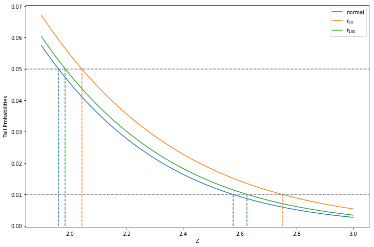
Hypothesis test: To test \(H_0: \beta_j = 0\) we form the standardized coefficient or Z-score: \[ z_j=\frac{\hat{B}_j}{\hat{\sigma}\sqrt{v_j}} \]

where \(v_j\) is the jth diagonal element of \((\mathbf{X}^T\mathbf{X})^{-1}\). Under the null hypothesis \(z_j\) is distributed as \(t_{N-p-1}\), and hence a large value of \(z_j\) will lead to rejection. If \(\hat{\sigma}\) is replaced by \(\sigma\) then \(z_j\) is a standard normal distribution. The difference between tail quantiles of a t-distribution and a standard normal become negligible as the sample size increases, see the Figure (3.3) below:

# Figure 3.3
%matplotlib inline

import matplotlib.pyplot as plt
import numpy as np
from scipy.stats import norm, t
   
fig = plt.figure(figsize = (12, 8))
axes = fig.add_subplot(1, 1, 1)

z = np.linspace(1.9, 3, 500)

normal_probabilities = 1 - norm.cdf(z) + norm.cdf(-z)
t_30_probabilities = 1 - t.cdf(z, 30) + t.cdf(-z, 30) 
t_100_probabilities = 1 - t.cdf(z, 100) + t.cdf(-z, 100) 

axes.plot(z, normal_probabilities, color='C0', label = 'normal')
axes.plot(z, t_30_probabilities, color='C1', label = '$t_{30}$')
axes.plot(z, t_100_probabilities, color='C2', label = '$t_{100}$')

xlim = axes.get_xlim()

for y in [0.01, 0.05]:
    axes.plot(xlim, [y, y], '--', color = 'gray', 
              scalex = False, scaley = False)

    for index, probs in enumerate([normal_probabilities, t_30_probabilities,
                                   t_100_probabilities]):
        x = z[np.abs(probs - y).argmin()]
        axes.plot([x, x], [0, y], '--', color = f"C{index}",
                  scalex = False, scaley = False)
    
axes.legend()
axes.set_xlabel('Z')
axes.set_ylabel('Tail Probabilities')
plt.show()

Test for the significance of groups of coefficients simultaneously: We use the F-statistics (3.13):

\[F=\frac{(RSS_0-RSS_1) / (p_1 - p_0)}{RSS_1/(N-p_1-1)}\]

Where \(RSS_1\) is for the bigger model with \(p_1+1\) parameters and \(RSS_0\) for the nested smaller model with \(p_0+1\) parameters. Under the null hypothesis that the smaller model is correct, the F statistic will have a \(F_{p_1-p_0,N-p_1-1}\) distribution. The \(z_j\) in (3.13) is equivalent to the F statistic for dropping the single coefficient \(\beta_j\) from the model.

Similarly, we can isolate \(\beta_j\) in (3.10) to obtain \(1-2\alpha\) confidence interval (3.14) \[(\hat{\beta_j} - z^{(1-\alpha)}v_j^{\frac{1}{2}}\hat{\sigma}, \hat{\beta_j} + z^{(1-\alpha)}v_j^{\frac{1}{2}}\hat{\sigma})\]

In a similar fashion we can obtain an approximate confidence set for the entire parameter vector \(\beta\) (3.15): \[ C_{\beta} = \{{\beta|(\hat{\beta}-\beta)^T\mathbf{X}^T\mathbf{X}(\hat{\beta}-\beta)} \le \hat{\sigma}^2{\chi_{p+1}^2}^{(1-\alpha)} \}\]

where \({\chi_{l}^2}^{(1-\alpha)}\) is the \(1-\alpha\) percentile of the chi-squared distribution of \(l\) degrees of freedom.